
From Scratch to Classifier: Building an Image Classifier with Minimal Data Using Transfer Learning
14 minute read
This tutorial is divided into two parts:
- Part 1: Creating a model
- Part 2: Deploying the model (Part 2)
Introduction
An image classifier is a machine learning model that sorts images into specific categories.
Building an image classifier from scratch usually needs a lot of data and training time. But with transfer learning and tools like Fastai and Hugging Face, you can quickly create a powerful image classifier even with just a small amount of data. In this blog, I’ll guide you through each step, showing you how to use these advanced tools to build a model that works well and is easy to use.
We’ll create a model to tell the difference between House Cats and Wild Cats—so you can avoid petting the wrong one. We’ll name it “TheCatClassifier”! By the end of this tutorial, you’ll have a working app that can accurately classify cats.
Prerequisites
- Basic understanding of Python programming.
- Familiarity with Jupyter Notebook or Google Colab.
- I’ll guide you through everything else.
For this tutorial, you don’t need a GPU. However, if you have one and want to use it to train your model, you can find instructions on setting up your GPU for training a machine learning model in my blog post here.
Step-by-Step Instructions
Installing ImageEngine
ImageEngine is a Python package I created for personal use. It allows you to easily download images from the web and installs other necessary libraries for this project. You can check out the project on GitHub and PyPI.
While ImageEngine is used here to download images, you can use any other method you prefer if you like.
pip install ImageEngine
(OPTIONAL) This step can be skipped if you are using Google Colab.
I recommend creating a virtual environment and then running the following command. You can follow the instructions in my article on setting up a GPU with PyTorch for creating a virtual environment using Anaconda, or use your preferred method.
Downloading CAT Images
Now, open Jupyter Notebook or Google Colab (familiarize yourself with it if you haven’t already) and import the following libraries.
from ImageEngine import searchWeb #Read more - https://github.com/jaypunekar/ImageEngine
from fastai.vision.all import *
Now, we will download images of house cat and wild cat from the internet.
# searchWeb function downloads images from Google, Duck Duck go and Bing

# "House cat" is the search string and "/cats/house_cat" is the folder where images are stored.
# 200 is the maximum number of images it will download from each search engine i.e. max 600.
# Occasionally, you might see warning/exceptions in between downloading process, you can ignore them.

searchWeb("different breed house cats", "cats/house_cats", 200)
searchWeb("lions", "cats/wild_cats", 50)
searchWeb("Tiger", "cats/wild_cats", 50)
searchWeb("Leopard", "cats/wild_cats", 50)
searchWeb("Wild cat", "cats/wild_cats", 50)

# We are using 4 prompts for wild cats because, just searching wild cats usually excludes Lions, Tigers etc.
# Path is a Fastai function it will add the path of cats folder to the "path" variable.
path = Path('cats')
Data to dataloaders
Creating a DataBlock
In Fastai, a DataBlock is a class used to prepare your data for training. It helps you organize and pre-process your data in a way that’s ready for model training. Essentially, it takes care of setting up your data pipeline, so you don’t have to handle the data preparation manually.
In simple terms, a DataBlock helps you efficiently manage your data and get it ready for training your model.
# To know more run the following code
??DataBlock
# DataBlock is like a template for creating dataloaders dataloaders
cats = DataBlock(
    blocks=(ImageBlock, CategoryBlock),
    get_items=get_image_files,
    splitter=RandomSplitter(valid_pct=0.2, seed=42), # This splits data into train(80%) and test(20%)
    get_y=parent_label, # Parent folder name will be Y
    item_tfms=Resize(128))
The data is typically divided into two parts: the training set and the testing set. In this case, 80% of the data is used for training, while the remaining 20% is reserved for testing. The model is trained on the training set and evaluated on the testing set.
Ideally, if you have enough data, it’s beneficial to split it into three sets: training, validation, and testing. The validation set is kept completely separate and unseen until the final evaluation. This separation is important because it helps prevent bias during the fine-tuning phase. By keeping the validation set isolated, you ensure that your model’s performance is assessed fairly after achieving good results on the test data.
For this tutorial, we will proceed without a separate validation set, but rest assured, your model will still deliver excellent results.
dls = cats.dataloaders(path)
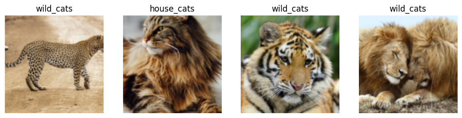
Remember, Fastai turns data into batches. To see the batch run the following command.
dls.valid.show_batch(max_n=4, nrows=1)
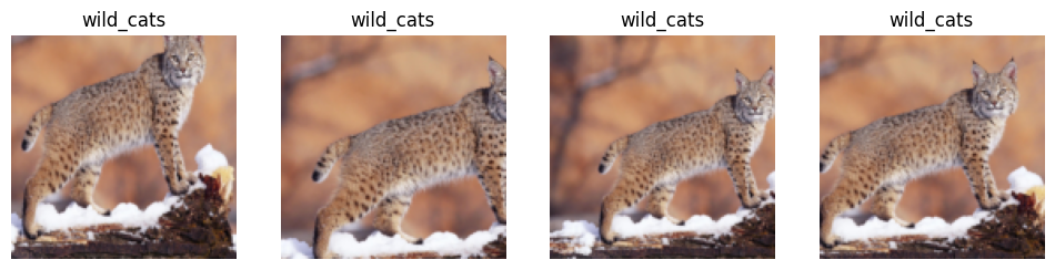
Next, we will apply transformations to the individual images to improve the model’s performance. One commonly used transformation is the RandomResizedCrop function. This function helps by randomly cropping and resizing the images, which can make the model more robust and improve its accuracy.
cats = cats.new(item_tfms=RandomResizedCrop(128, min_scale=0.3))
# If you have small data then add a parameter bs and set it to a small number, eg. dataloaders(path, bs=5)
dls = cats.dataloaders(path)
dls.train.show_batch(max_n=4, nrows=1, unique=True)
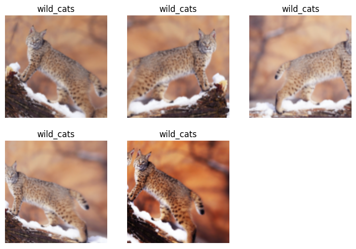
Data Augmentation
Fastai creates batches to feed into GPU(default 64).
Now, we’ll transform the image batches. This process is known as Data Augmentation. Data augmentation helps improve the model’s generalization by applying random transformations to the images.
To apply data augmentation, run the following command:
# aug_transforms is a set of standard augmentations that fastai provides
cats = cats.new(item_tfms=Resize(128), batch_tfms=aug_transforms(mult=2))
dls = cats.dataloaders(path, bs=5)
dls.train.show_batch(max_n=8, nrows=2, unique=True)
Training Your Model
To integrate both image resizing and data augmentation, use the following code:
# putting both the approaches together
cats = cats.new(
    item_tfms=RandomResizedCrop(224, min_scale=0.5),
    batch_tfms=aug_transforms())
dls = cats.dataloaders(path, bs=5)
# bs=5 is batch size, default batch size is 64, but if you don't have enough data
# it's better to reduce it.
Now, we’re going to train the model using a pre-trained model called “resnet18” as the base.
You don’t need to worry about the details too much. This approach is known as transfer learning. It involves using a pre-trained model and modifying its head node to suit your specific task. ResNet is a popular choice for vision models due to its proven performance in various image classification tasks.
By leveraging a pre-trained model, you can benefit from the features learned from a large dataset, which can significantly speed up the training process and improve accuracy.
# I have explained the parameters below
learn = vision_learner(dls, resnet18, metrics=error_rate)
learn.fine_tune(4)
| epoch | train_loss | valid_loss | error_rate | time |
|---|---|---|---|---|
| 0 | 0.674404 | 0.270994 | 0.077381 | 01:09 |
| epoch | train_loss | valid_loss | error_rate | time |
|---|---|---|---|---|
| 0 | 0.521202 | 0.164568 | 0.041667 | 01:22 |
| 1 | 0.467215 | 0.282850 | 0.125000 | 01:22 |
| 2 | 0.386020 | 0.050403 | 0.023810 | 01:22 |
| 3 | 0.299196 | 0.066655 | 0.023810 | 01:22 |
In less than 2 minutes, we achieved an error rate of less than 0.03 (3%).
The metrics parameter in the training process indicates how well the model is performing, essentially showing the error rate. It’s important to note that metrics are different from “loss”. While “loss” is used internally by the neural network to evaluate its performance, it’s not meant for human interpretation. On the other hand, metrics are designed to help us understand the model’s performance in more relatable terms.
You might wonder why we are using the fine_tune method instead of fit. The reason is that fine_tune adjusts a pre-trained model (like ResNet18 in this case) to our specific task, while fit would train the model from scratch, ignoring the benefits of the pre-trained model. Fastai does offer a fit method, but for transfer learning, fine_tune is the appropriate choice.
To further evaluate the model’s performance and identify where it might be going wrong, we will create a Confusion Matrix.
interp = ClassificationInterpretation.from_learner(learn)
interp.plot_confusion_matrix()
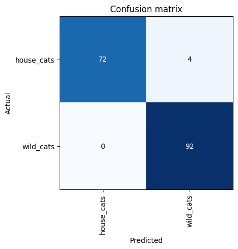
We can see that only 4 images have been classified incorrectly. To get more details and understand where the model might be making mistakes, run the following command:
interp.plot_top_losses(5, nrows=1, figsize=(25, 4))
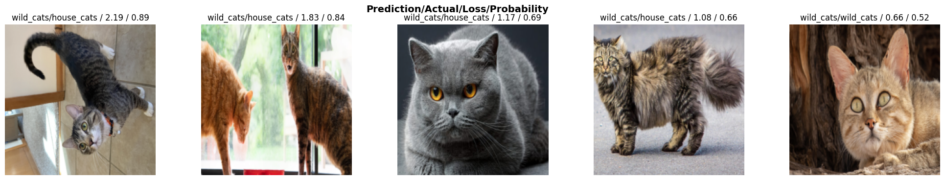
We can see that with very little training time and data, we achieve over 97% accuracy on our model. It’s impressive considering we haven’t cleaned or thoroughly examined our data, yet we are still getting exceptional results.
The next question is: how do we use this model in an application, whether it’s a mobile app, web app, or any other type of application? To do this, we will export the model in pickle format. I’ll show you how this works. But first, let’s test our model.
Testing created model with random data
Now, it’s time to test our model with random images from the internet. We will also include some non-cat images to see how the model performs with data it hasn’t seen before.
# Run pip install fastbook
from fastbook import *
uploader = widgets.FileUpload()
uploader
FileUpload(value={}, description='Upload')
img = PILImage.create(uploader.data[0])
whichCat,_,probs = learn.predict(img)
print(whichCat, ", ", probs)
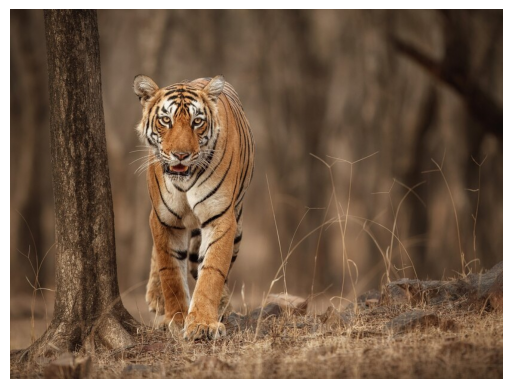
Since we can’t upload images directly in this blog, I’ve taken an image of a tiger from the internet and will display it using Matplotlib. This allows us to visualize the image and test how our model handles it.
Here’s how you can display the image using Matplotlib:
import matplotlib.pyplot as plt
import matplotlib.image as mpimg
import requests
from io import BytesIO

# URL of the image
url = "https://img.freepik.com/free-photo/amazing-bengal-tiger-nature_475641-1189.jpg?w=826&t=st=1725798003~exp=1725798603~hmac=51a8f3a4146639871a6ad8f701cb24cc3be6f122875332d2a358feff5b81e234"

# Fetch the image
response = requests.get(url)
img = mpimg.imread(BytesIO(response.content), format='jpg')

# Display the image
plt.imshow(img)
plt.axis('off')  # Hide axis
plt.show()
To make a prediction using our model, we use the learn.predict(img) method. This method returns three objects: the predicted class label, the prediction index, and the probabilities for each class. You can name these variables however you like. In the example provided, whichCat represents the predicted class label (which corresponds to the name of the parent folder), and probs contains the probabilities for each possible class.
Here’s the code to get the prediction and probabilities:
whichCat,_,probs = learn.predict(img)
print(whichCat, ", ", probs)
wild_cats , tensor([0.0011, 0.9989])
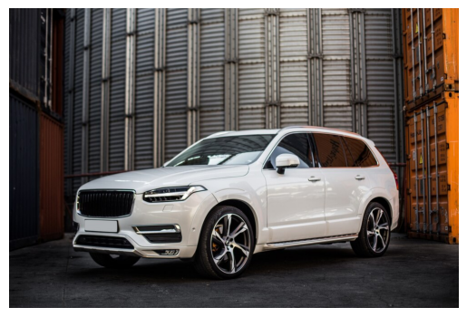
Now, let’s test this with a random image of a car and see what the prediction reveals:
# URL of the image
url = "https://img.freepik.com/free-photo/white-offroader-jeep-parking_114579-4007.jpg?w=996&t=st=1725798998~exp=1725799598~hmac=f951a0affff110c507c31780983e6c8d6eacd7d81304bb8eec346227882ea3c9"

# Fetch the image
response = requests.get(url)
img = mpimg.imread(BytesIO(response.content), format='jpg')

# Display the image
plt.imshow(img)
plt.axis('off')  # Hide axis
plt.show()
whichCat,_,probs = learn.predict(img)
print(whichCat, ", ", probs)
wild_cats , tensor([0.4883, 0.5117])
As you can see, this model will attempt to classify any given image into “wild” or “house” cats. It’s important to note that this behavior is not a bug but rather a limitation of how this type of model is designed. We won’t be addressing this issue in this blog, but you can read the Fastai docs for more information and potential workarounds.
Exporting the model
To export the model, use the following command:
learn.export() # learn.export("name_of_model.pkl")
# Check if the file exist
path = Path()
path.ls(file_exts='.pkl')
The learn.export() method saves the model as export.pkl in the current directory by default. If you want to use a custom name for the saved model, specify it as a string parameter, making sure to include the .pkl extension. For example, learn.export('my_custom_model.pkl') will save the model as my_custom_model.pkl.
Additionally, you can provide a full path to save the model in a specific directory. For instance, learn.export('model/mymodel.pkl') will create a model directory (if it doesn’t already exist) in your current directory and save the model as mymodel.pkl inside that directory.
If you use learn.export() with no parameters or with 'export.pkl', the model will be saved as export.pkl in the current directory.
To load the saved model, use the following command:
learn = load_learner('path_to_model/export.pkl')
To load the saved model, use the following command:
learn_inf = load_learner('export.pkl')
Now, learn_inf has all the functionality of the original learn object. You can test it using the img variable (which contains the car image) as follows:
img, idx, probs = learn_inf.predict(img)
print(img, idx, probs)
wild_cats tensor(1) tensor([0.4883, 0.5117])
We have successfully exported the trained model, and now it’s time to deploy it. You can find the deployment process in Part 2 of this blog series.
Check out Part 2 to learn how to deploy your model and make it accessible on the web.
Limitations of this Model
Let’s say we really were rolling out a cat detection system that will be attached to video cameras around campsites in national parks and will warn campers of incoming cats. If we used a model trained with the dataset we downloaded, there would be all kinds of problems in practice, such as these:
- Working with video data instead of images
- Handling nighttime images, which may not appear in this dataset
- Dealing with low-resolution camera images
- Ensuring results are returned fast enough to be useful in practice
- Recognizing cats in positions that are rarely seen in photos that people post online (for example from behind, partially covered by bushes, or a long way away from the camera)
A big part of the issue is that the kinds of photos that people are most likely to upload to the internet are the kinds of photos that do a good job of clearly and artistically displaying their subject matter—which isn’t the kind of input this system is going to be getting. So, we may need to do a lot of our own data collection and labeling to cre‐ ate a useful system.
Conclusion
In this tutorial, we demonstrated how to quickly create an image classifier using transfer learning with Fastai. We started by setting up our environment, downloading and preparing the data, and training a model to distinguish between house cats and wild cats. With minimal data and training time, we achieved impressive results, thanks to the power of transfer learning.
By exporting the trained model, we made it ready for deployment. In the next part, we’ll cover how to deploy this model so that it can be used in real-world applications. Stay tuned to see how you can put your model to work on the web!